Prototype - Time Series Analysis

1. Load Packages

pacman::p_load(tidyverse, ggiraph, reshape, ggthemes, 
               gganimate, plotly, scales, ggHoriPlot, ggrepel,
               CGPfunctions, ggTimeSeries, datagovsgR, neaSG)

2. Import Data

Temp_YM <- readRDS("data/temperature.rds")
Rainfall_YM <- readRDS("data/rainfall.rds")

3. Overview

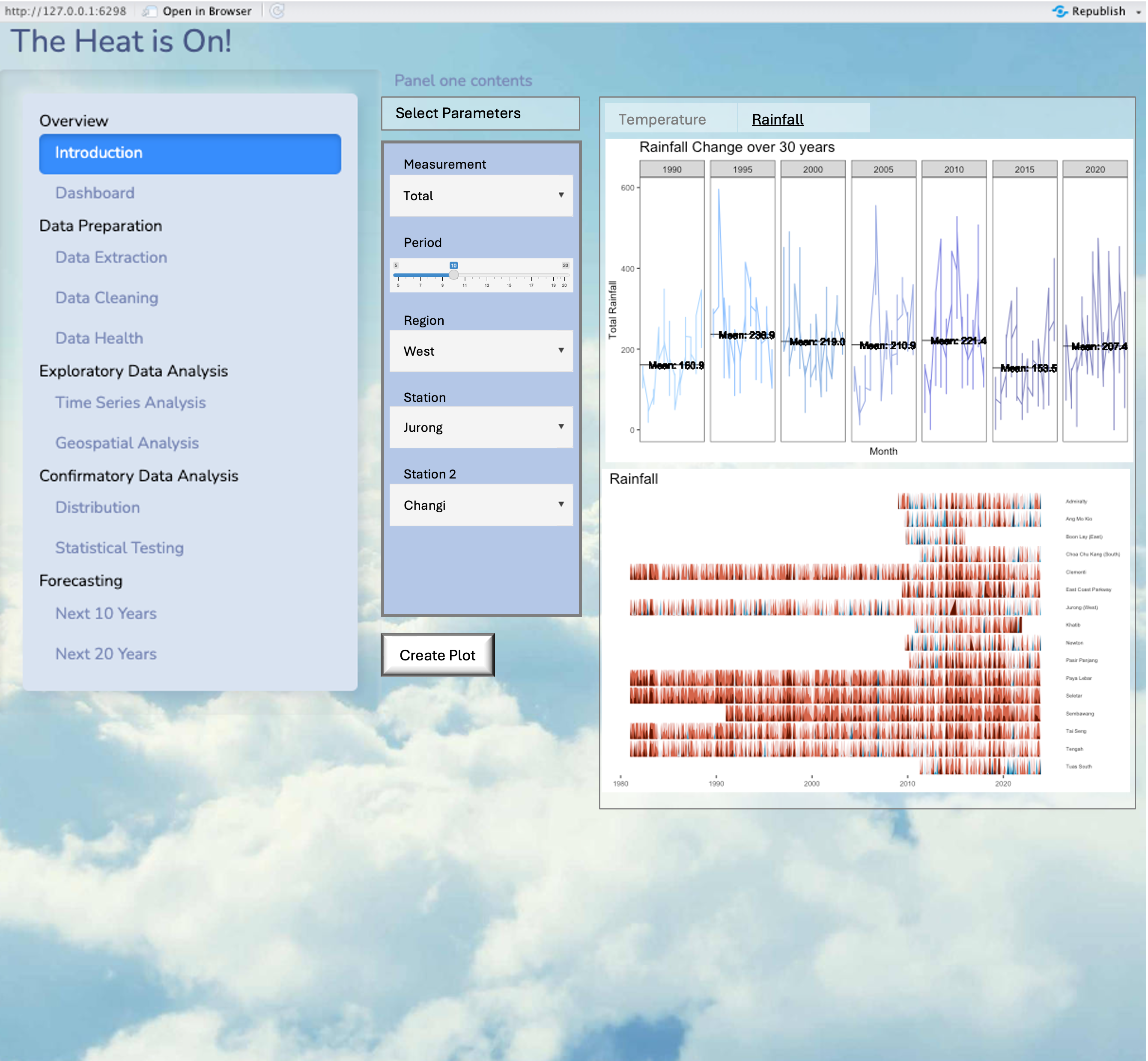
3.1 Dashboard

Prototype

Total Stations

station_count <- Temp_YM %>%
  summarise(Station_Count = n_distinct(Station))
station_count

# A tibble: 1 × 1
  Station_Count
          <int>
1            18

Mean Temperature

mean_temperature <- Temp_YM %>%
  summarise(Mean_Temperature = round(mean(MeanTemp, na.rm = TRUE), 1))
mean_temperature

# A tibble: 1 × 1
  Mean_Temperature
             <dbl>
1             27.7

Total Rainfall

mean_totalrainfall <- Rainfall_YM %>%
  summarise(Mean_Total_Rainfall = round(mean(TotalRainfall, na.rm = TRUE), 1))
mean_totalrainfall

# A tibble: 1 × 1
  Mean_Total_Rainfall
                <dbl>
1                206.

3.2 Live Weather Forecast

Weather Forecast

This functions calls upon the weather forecast API from data.gov.sg and returns a data frame con- taining different metrics of the forecast. 2-hour, 24-hour and 4-day forecasts are availible. This data provided by the API is updated half-hourly.

current_time <- Sys.time()
formatted_date <- format(current_time, "%Y-%m-%d")
formatted_time <- format(current_time, "%H:%M:%S")
formatted_datetime <- paste(formatted_date, formatted_time, sep = "T")

weather_forecast(formatted_datetime)

                      area forecast
1               Ang Mo Kio   Cloudy
2                    Bedok   Cloudy
3                   Bishan   Cloudy
4                 Boon Lay   Cloudy
5              Bukit Batok   Cloudy
6              Bukit Merah   Cloudy
7            Bukit Panjang   Cloudy
8              Bukit Timah   Cloudy
9  Central Water Catchment   Cloudy
10                  Changi   Cloudy
11           Choa Chu Kang   Cloudy
12                Clementi   Cloudy
13                    City   Cloudy
14                 Geylang   Cloudy
15                 Hougang   Cloudy
16             Jalan Bahar   Cloudy
17             Jurong East   Cloudy
18           Jurong Island   Cloudy
19             Jurong West   Cloudy
20                 Kallang   Cloudy
21            Lim Chu Kang   Cloudy
22                  Mandai   Cloudy
23           Marine Parade   Cloudy
24                  Novena   Cloudy
25               Pasir Ris   Cloudy
26              Paya Lebar   Cloudy
27                 Pioneer   Cloudy
28            Pulau Tekong   Cloudy
29              Pulau Ubin   Cloudy
30                 Punggol   Cloudy
31              Queenstown   Cloudy
32                 Seletar   Cloudy
33               Sembawang   Cloudy
34                Sengkang   Cloudy
35                 Sentosa   Cloudy
36               Serangoon   Cloudy
37        Southern Islands   Cloudy
38            Sungei Kadut   Cloudy
39                Tampines   Cloudy
40                 Tanglin   Cloudy
41                  Tengah   Cloudy
42               Toa Payoh   Cloudy
43                    Tuas   Cloudy
44         Western Islands   Cloudy
45 Western Water Catchment   Cloudy
46               Woodlands   Cloudy
47                  Yishun   Cloudy

Air Temperature

get_airtemp(formatted_date, formatted_date)

[1] "2024-04-01"
[1] "2024-04-01"

                      timestamp readings.station_id readings.value
                         <char>              <char>          <num>
   1: 2024-04-01T00:01:00+08:00                S109           28.0
   2: 2024-04-01T00:02:00+08:00                S109           28.0
   3: 2024-04-01T00:03:00+08:00                S109           28.0
   4: 2024-04-01T00:04:00+08:00                S109           28.0
   5: 2024-04-01T00:05:00+08:00                S109           28.0
  ---                                                             
1410: 2024-04-01T23:31:00+08:00                S109           28.8
1411: 2024-04-01T23:32:00+08:00                S109           28.7
1412: 2024-04-01T23:33:00+08:00                S109           28.7
1413: 2024-04-01T23:34:00+08:00                S109           28.7
1414: 2024-04-01T23:35:00+08:00                 S43           29.4
      readings.station_id.1 readings.value.1 readings.station_id.2
                     <char>            <num>                <char>
   1:                  S117             28.8                   S50
   2:                  S117             28.8                   S50
   3:                  S117             28.8                   S50
   4:                  S117             28.8                   S50
   5:                  S117             28.8                   S50
  ---                                                             
1410:                  S117             29.2                   S50
1411:                  S117             29.2                   S50
1412:                  S117             29.2                   S50
1413:                  S117             29.2                   S50
1414:                   S44             29.2                  S111
      readings.value.2 readings.station_id.3 readings.value.3
                 <num>                <char>            <num>
   1:             27.6                  S107             29.3
   2:             27.6                  S107             29.3
   3:             27.6                  S107             29.4
   4:             27.5                  S107             29.4
   5:             27.5                  S107             29.4
  ---                                                        
1410:             28.4                  S107             29.4
1411:             28.4                  S107             29.4
1412:             28.4                  S107             29.4
1413:             28.4                  S107             29.4
1414:             28.4                  S115             29.4
      readings.station_id.4 readings.value.4 readings.station_id.5
                     <char>            <num>                <char>
   1:                   S43             28.8                   S44
   2:                   S43             28.7                   S44
   3:                   S43             28.7                   S44
   4:                   S43             28.8                   S44
   5:                   S43             28.8                   S44
  ---                                                             
1410:                   S44             29.2                  S121
1411:                   S43             29.4                   S44
1412:                   S43             29.4                   S44
1413:                   S43             29.4                   S44
1414:                  <NA>               NA                  <NA>
      readings.value.5 readings.station_id.6 readings.value.6
                 <num>                <char>            <num>
   1:             27.4                  S121             27.1
   2:             27.4                  S121             27.0
   3:             27.4                  S121             27.1
   4:             27.4                  S121             27.1
   5:             27.4                  S121             27.0
  ---                                                        
1410:             28.6                  S111             28.4
1411:             29.2                  S121             28.6
1412:             29.2                  S121             28.6
1413:             29.2                  S121             28.6
1414:               NA                  <NA>               NA
      readings.station_id.7 readings.value.7 readings.station_id.8
                     <char>            <num>                <char>
   1:                  S111             28.1                   S24
   2:                  S111             28.1                   S24
   3:                  S111             28.1                  S115
   4:                  S111             28.1                  S115
   5:                  S111             28.1                  S115
  ---                                                             
1410:                   S60             29.1                   S24
1411:                  S111             28.4                   S60
1412:                  S111             28.4                   S60
1413:                  S111             28.4                   S60
1414:                  <NA>               NA                  <NA>
      readings.value.8 readings.station_id.9 readings.value.9
                 <num>                <char>            <num>
   1:             28.2                  S116             28.8
   2:             28.2                  S116             28.8
   3:             28.8                   S24             28.2
   4:             28.7                   S24             28.2
   5:             28.7                   S24             28.2
  ---                                                        
1410:             29.2                  S116             29.2
1411:             29.1                   S24             29.1
1412:             29.1                  S115             29.5
1413:             29.1                  S115             29.5
1414:               NA                  <NA>               NA
      readings.station_id.10 readings.value.10 readings.station_id.11
                      <char>             <num>                 <char>
   1:                   S104              27.3                   <NA>
   2:                   S104              27.3                   <NA>
   3:                   S116              28.8                   S104
   4:                   S116              28.7                   S104
   5:                   S116              28.7                   S104
  ---                                                                
1410:                   S104              28.8                   <NA>
1411:                   S116              29.2                   S104
1412:                    S24              29.1                   S116
1413:                    S24              29.1                   S116
1414:                   <NA>                NA                   <NA>
      readings.value.11 readings.station_id.12 readings.value.12
                  <num>                 <char>             <num>
   1:                NA                   <NA>                NA
   2:                NA                   <NA>                NA
   3:              27.3                   <NA>                NA
   4:              27.3                   <NA>                NA
   5:              27.2                   <NA>                NA
  ---                                                           
1410:                NA                   <NA>                NA
1411:              28.8                   <NA>                NA
1412:              29.2                   S104              28.8
1413:              29.2                   S104              28.7
1414:                NA                   <NA>                NA

latest_airtemp <- head(get_airtemp(formatted_date, formatted_date), n = 1)

[1] "2024-04-01"
[1] "2024-04-01"

column_names <- paste0("readings.value.", 1:12)
values <- sapply(column_names, function(col) latest_airtemp[[col]])
average_value <- mean(values, na.rm = TRUE)
print(average_value)

[1] 28.14

Ultra-violet Index

This functions calls upon the UVI API from data.gov.sg and returns a data frame of the different measures of the UVI across Singapore and returns the closest UVI value presently and for the past few hours. This data provided by the API is updated hourly.

uvi(formatted_datetime)

   value                 timestamp
1      0 2024-04-01T19:00:00+08:00
2      1 2024-04-01T18:00:00+08:00
3      3 2024-04-01T17:00:00+08:00
4      5 2024-04-01T16:00:00+08:00
5      6 2024-04-01T15:00:00+08:00
6      8 2024-04-01T14:00:00+08:00
7      7 2024-04-01T13:00:00+08:00
8      6 2024-04-01T12:00:00+08:00
9      4 2024-04-01T11:00:00+08:00
10     2 2024-04-01T10:00:00+08:00
11     1 2024-04-01T09:00:00+08:00
12     0 2024-04-01T08:00:00+08:00
13     0 2024-04-01T07:00:00+08:00

# Display only the latest timestamp
# Retrieve the UV index for the latest timestamp
latest_uvi <- head(uvi(formatted_datetime), n = 1)
print(latest_uvi$value)

[1] 0

3.3 Animation

Temperature

MeanTemp_Year <- Temp_YM %>% 
  group_by(Year) %>% 
  summarise(MeanTemp_Year = round(mean(MeanTemp, na.rm = TRUE), 1))

Temp_YM <- left_join(Temp_YM, MeanTemp_Year, by = c("Year"))

glimpse(Temp_YM)

Rows: 3,715
Columns: 9
$ Station       <chr> "Admiralty", "Admiralty", "Admiralty", "Admiralty", "Adm…
$ Region        <chr> "North", "North", "North", "North", "North", "North", "N…
$ Year          <dbl> 2009, 2009, 2009, 2009, 2009, 2009, 2009, 2009, 2009, 20…
$ Month         <ord> Jan, Feb, Mar, Apr, May, Jun, Jul, Aug, Sep, Oct, Nov, D…
$ Date          <date> 2009-01-01, 2009-02-01, 2009-03-01, 2009-04-01, 2009-05…
$ MeanTemp      <dbl> 26.3, 26.8, 26.9, 28.1, 28.5, 28.9, 28.1, 28.1, 28.3, 28…
$ MaxTemp       <dbl> 31.9, 33.4, 34.5, 35.1, 34.7, 34.7, 33.7, 33.6, 34.3, 34…
$ MinTemp       <dbl> 23.3, 23.0, 22.2, 23.7, 21.8, 23.7, 22.5, 22.7, 23.1, 22…
$ MeanTemp_Year <dbl> 27.6, 27.6, 27.6, 27.6, 27.6, 27.6, 27.6, 27.6, 27.6, 27…

ggplot(Temp_YM, aes(x = Month, y = MeanTemp)) +
  geom_point(aes(color = MeanTemp), alpha = 0.5, size = 4, show.legend = FALSE) +
  scale_color_gradient(low = "darkorange", high = "darkred") +
  geom_boxplot(aes(y = MeanTemp_Year), width = 0.8, color = "darkgoldenrod1") +
  scale_size(range = c(2, 12)) +
  labs(title = 'Mean Temperature, 1986-2023 \nYear: {frame_time}', 
       x = 'Month', 
       y = 'Mean Temperature (°C)') +
  transition_time(as.integer(Year)) + 
  ease_aes('linear') +
  theme(legend.position = "right",
        panel.grid.major = element_blank(),
        panel.grid.minor = element_blank()) +
  guides(color = guide_legend(title = "Average Temperature", override.aes = list(color = "grey", linetype = "dashed"))) +
  theme_hc()

Rainfall

TotalRainfall_Year <- Rainfall_YM %>% 
  group_by(Year) %>% 
  summarise(MeanRainfall_Year = round(mean(TotalRainfall, na.rm = TRUE), 1))
Rainfall_YM <- left_join(Rainfall_YM, TotalRainfall_Year, by = c("Year"))
glimpse(Rainfall_YM)

Rows: 5,547
Columns: 10
$ Station           <chr> "Admiralty", "Admiralty", "Admiralty", "Admiralty", …
$ Region            <chr> "North", "North", "North", "North", "North", "North"…
$ Year              <dbl> 2009, 2009, 2009, 2009, 2009, 2009, 2009, 2009, 2009…
$ Month             <ord> Jan, Feb, Mar, Apr, May, Jun, Jul, Aug, Sep, Oct, No…
$ Date              <date> 2009-01-01, 2009-02-01, 2009-03-01, 2009-04-01, 200…
$ TotalRainfall     <dbl> 0.8, 148.0, 348.0, 148.8, 205.6, 92.0, 103.0, 90.2, …
$ TotalRainfall30   <dbl> 0, 0, 0, 0, 0, 0, 0, 0, 0, 0, 0, 0, 0, 0, 0, 0, 0, 0…
$ TotalRainfall60   <dbl> 0, 0, 0, 0, 0, 0, 0, 0, 0, 0, 0, 0, 0, 0, 0, 0, 0, 0…
$ TotalRainfall120  <dbl> 0, 0, 0, 0, 0, 0, 0, 0, 0, 0, 0, 0, 0, 0, 0, 0, 0, 0…
$ MeanRainfall_Year <dbl> 172.5, 172.5, 172.5, 172.5, 172.5, 172.5, 172.5, 172…

ggplot(Rainfall_YM, aes(x = Month, y = TotalRainfall)) +
  geom_point(aes(color = TotalRainfall), shape = 17, alpha = 0.5, size = 4, show.legend = FALSE) +
  scale_color_gradient(low = "lightblue", high = "darkblue") +
  geom_boxplot(aes(y = MeanRainfall_Year), width = 0.8, color = "cornflowerblue") +
  scale_size(range = c(2, 12)) +
  labs(title = 'Total Rainfall, 1986-2023 \nYear: {frame_time}', 
       x = 'Month', 
       y = 'Total Rainfall (mm)') +
  transition_time(as.integer(Year)) + 
  ease_aes('linear') +
  theme(legend.position = "right",
        panel.grid.major = element_blank(),
        panel.grid.minor = element_blank()) +
  guides(color = guide_legend(title = "Total Rainfall", override.aes = list(color = "grey", linetype = "dashed"))) +
  theme_hc()

4. Time Series Analysis

Prototype

Temperature

Rainfall

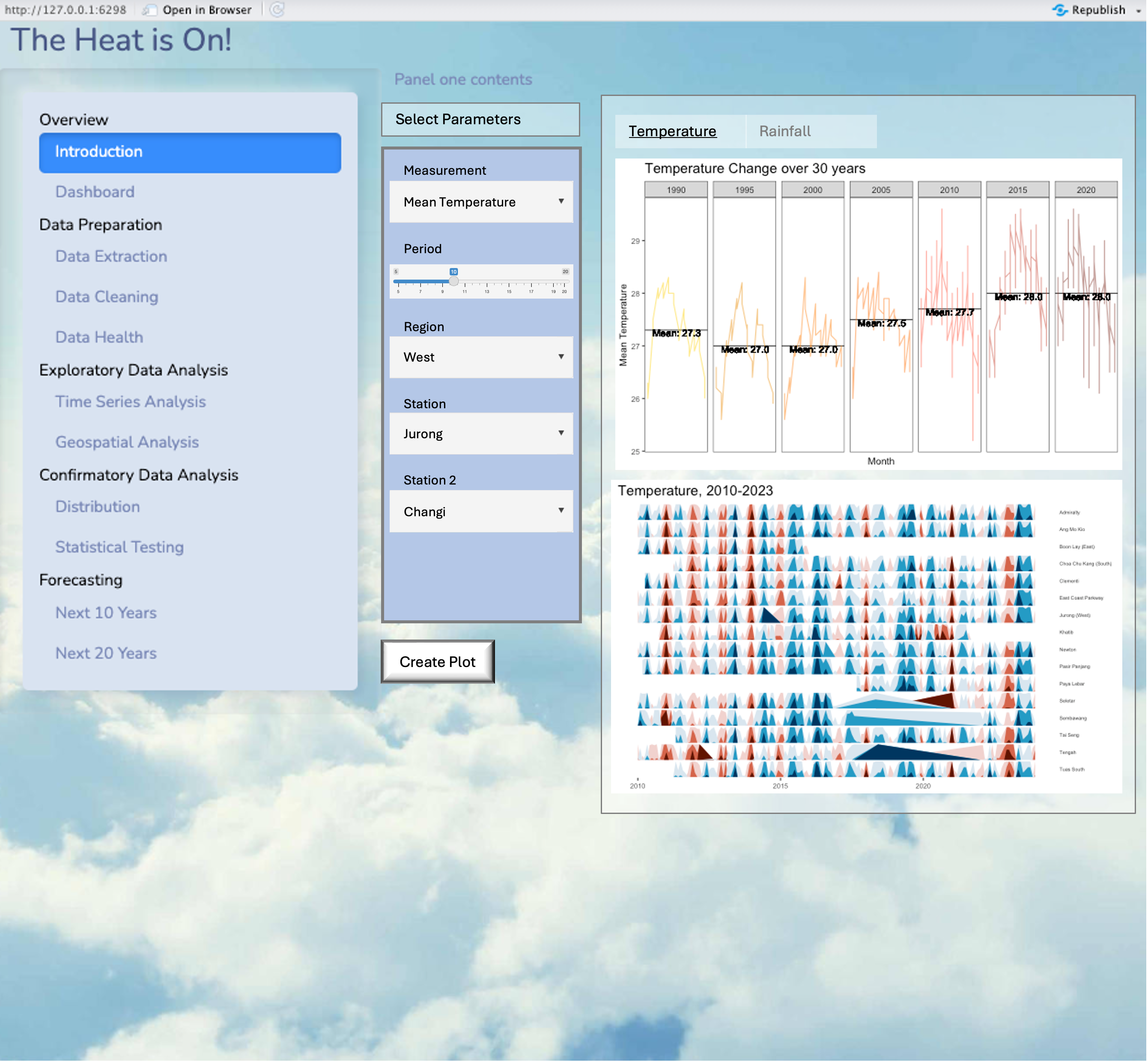
4.1 Cycle Plot

# Selecting 5 years
selection <- c(1990, 1995, 2000, 2005, 2010, 2015, 2020)

# Filtering the dataframe for the selected years
cycle_input <- Temp_YM %>%
  filter(Year %in% selection)

# Define darker pastel colors
palette <- c("gold1", "orange2", "darkorange", "darkorange1", "tomato1", "tomato3", "tomato4")

# Plot with darker pastel colors
ggplot(data = cycle_input) +
  geom_hline(data = cycle_input,
             aes(yintercept = `MeanTemp_Year`),
             color = "black",
             alpha = 1.0,
             size = 0.4) +
  geom_line(aes(x = Month,
                y = MeanTemp,
                group = Year,
                color = as.factor(Year),
                alpha = 0.6)) +
  geom_text(data = cycle_input,
            aes(x = 1, y = MeanTemp_Year - 0.05, label = paste0("Mean: ", sprintf("%.1f", MeanTemp_Year))),
            hjust = -0.1, vjust = 0.5, color = "black", size = 3.5) +
  facet_grid(~Year) + 
  labs(x = "Month",
       y = "Mean Temperature") +
  ggtitle("Temperature Change over 30 years") +
  theme_bw() +
  theme(legend.position = "none",
        axis.text.x = element_blank(),
        axis.ticks.x = element_blank(),
        axis.title = element_text(size = 10),
        title = element_text(size =12),
        axis.text.y = element_text(size = 8),
        panel.grid.major = element_blank(),
        panel.grid.minor = element_blank()) +
  scale_color_manual(values = palette)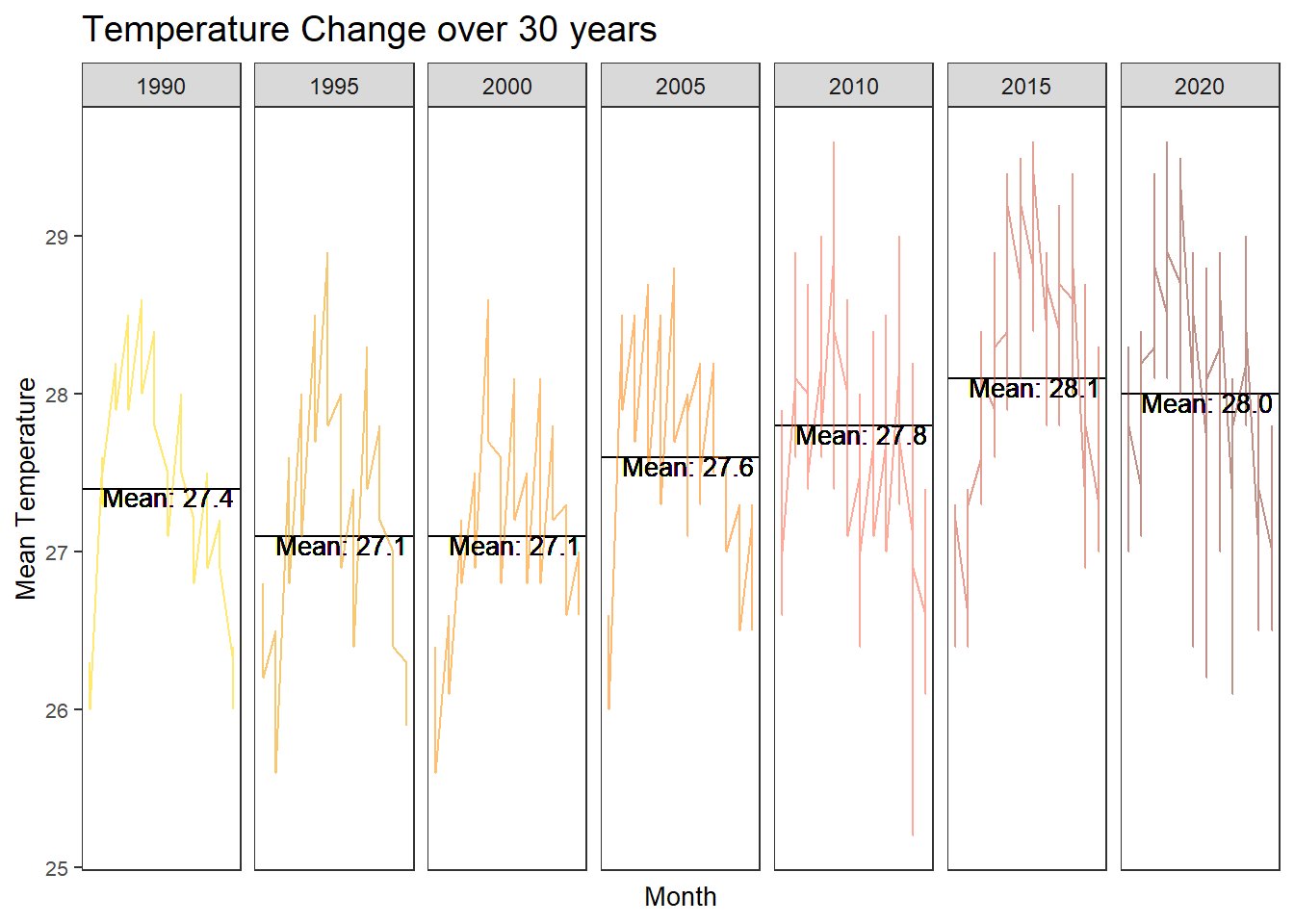

# Filtering the dataframe for the selected years
cycle_input <- Rainfall_YM %>%
  filter(Year %in% selection)

# Define darker pastel colors
palette <- c("steelblue1", "dodgerblue", "dodgerblue3", "royalblue3", "blue3", "blue4", "darkblue")

# Plot with darker pastel colors
ggplot(data = cycle_input) +
  geom_hline(data = cycle_input,
             aes(yintercept = `MeanRainfall_Year`),
             color = "black",
             alpha = 1.0,
             size = 0.4) +
  geom_line(aes(x = Month,
                y = TotalRainfall,
                group = Year,
                color = as.factor(Year),
                alpha = 0.6)) +
  geom_text(data = cycle_input,
            aes(x = 1, y = MeanRainfall_Year - 0.05, label = paste0("Mean: ", sprintf("%.1f", MeanRainfall_Year))),
            hjust = -0.1, vjust = 0.5, color = "black", size = 3.5) +
  facet_grid(~Year) + 
  labs(x = "Month",
       y = "Total Rainfall") +
  ggtitle("Rainfall Change over 30 years") +
  theme_bw() +
  theme(legend.position = "none",
        axis.text.x = element_blank(),
        axis.ticks.x = element_blank(),
        axis.title = element_text(size = 10),
        title = element_text(size =12),
        axis.text.y = element_text(size = 8),
        panel.grid.major = element_blank(),
        panel.grid.minor = element_blank()) +
  scale_color_manual(values = palette)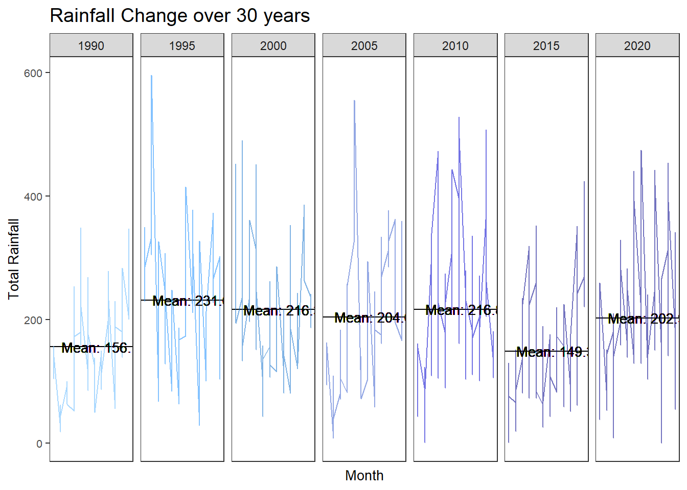

Transformation to Shiny App

UI

UI(fluidPage(
  
  titlePanel("Temperature and Rainfall Analysis"),
  
  sidebarLayout(
    sidebarPanel(
      selectInput("data", "Select Data:",
                  choices = c("Temperature", "Rainfall")),
      sliderInput("period", "Select Period:",
                  min = 1980, max = 2023, value = c(1990, 2020)),
      selectInput("region", "Select Region:",
                  choices = c("Region A", "Region B", "Region C")),
      selectInput("station", "Select Station:",
                  choices = c("Station 1", "Station 2", "Station 3"))
    ),
    mainPanel(
      plotOutput("plot")
    )
  )
))

Server

Server(function(input, output) {
  
  output$plot <- renderPlot({
    # Filter data based on user inputs
    filtered_data <- filter_data(input$data, input$period[1], input$period[2],
                                 input$region, input$station)
    
    # Plotting based on filtered data
    ggplot(filtered_data) +
      geom_line(aes(x = Month, y = MeanTemp, group = Year, color = as.factor(Year)),
                alpha = 0.6) +
      labs(x = "Month", y = ifelse(input$data == "Temperature", "Mean Temperature", "Total Rainfall")) +
      ggtitle(ifelse(input$data == "Temperature", "Temperature Change over Time", "Rainfall over Time")) +
      theme_minimal()
  })
  
  # Function to filter data based on user inputs
  filter_data <- function(data_type, start_year, end_year, region, station) {
    # Your data filtering logic here based on user inputs
    # For demonstration, let's assume you have a dataframe called "data"
    # with columns: Month, Year, MeanTemp, TotalRainfall, Region, Station
    
    filtered_data <- data %>%
      filter(Year >= start_year, Year <= end_year,
             Region == region, Station == station)
    
    if (data_type == "Temperature") {
      return(filtered_data %>% select(Month, Year, MeanTemp))
    } else {
      return(filtered_data %>% select(Month, Year, TotalRainfall))
    }
  }
  
})

4.2 Slope Graph

Temp_YM %>% 
  mutate(Year = factor(Year), 
         Station = factor(Station)) %>%
  filter(Year %in% c(2017, 2023)) %>%
  newggslopegraph(Year, MeanTemp_Year, Station,
                Title = "Temperature",
                SubTitle = "1983-2023",
                Caption = "Taught by: Dr. Kam Tin Seong")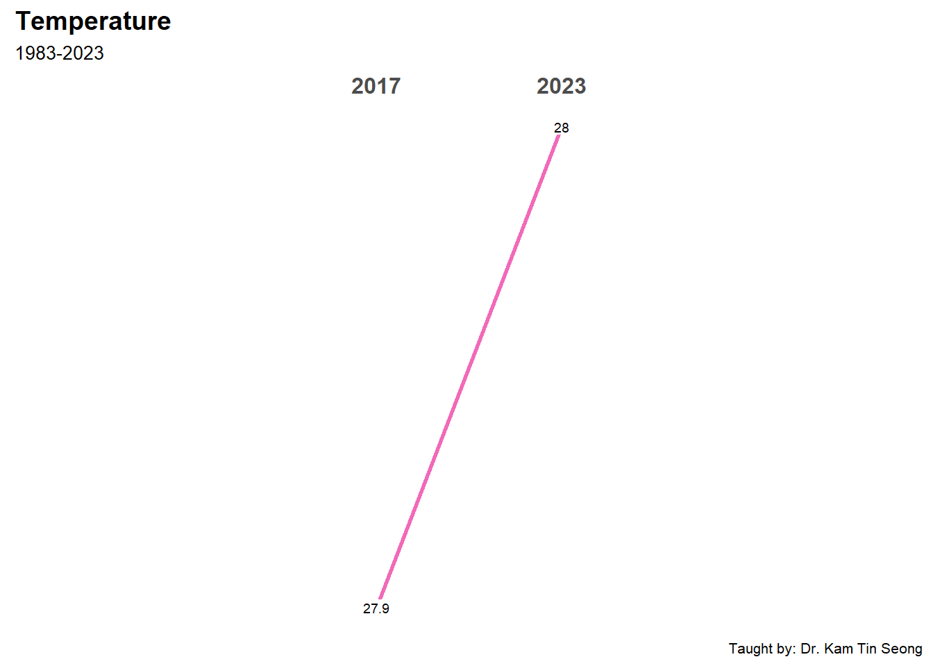

Temp_slope <- Temp_YM %>%
  select(Station, Year, MeanTemp_Year) %>%
  distinct()

Temp_slope <- Temp_slope %>%
  mutate(Year = factor(Year))

Temp_slope_filtered <- Temp_slope %>%
  filter(Year %in% c(2017, 2023))

slope_plot <- newggslopegraph(data = Temp_slope_filtered,
                              Year, MeanTemp_Year, Station,
                              Title = "Temperature",
                              SubTitle = "2017-2023",
                              Caption = "Taught by: Dr. Kam Tin Seong")

slope_plot + geom_text_repel(aes(label = Station), size = 3, box.padding = 0.5, max.overlaps = Inf)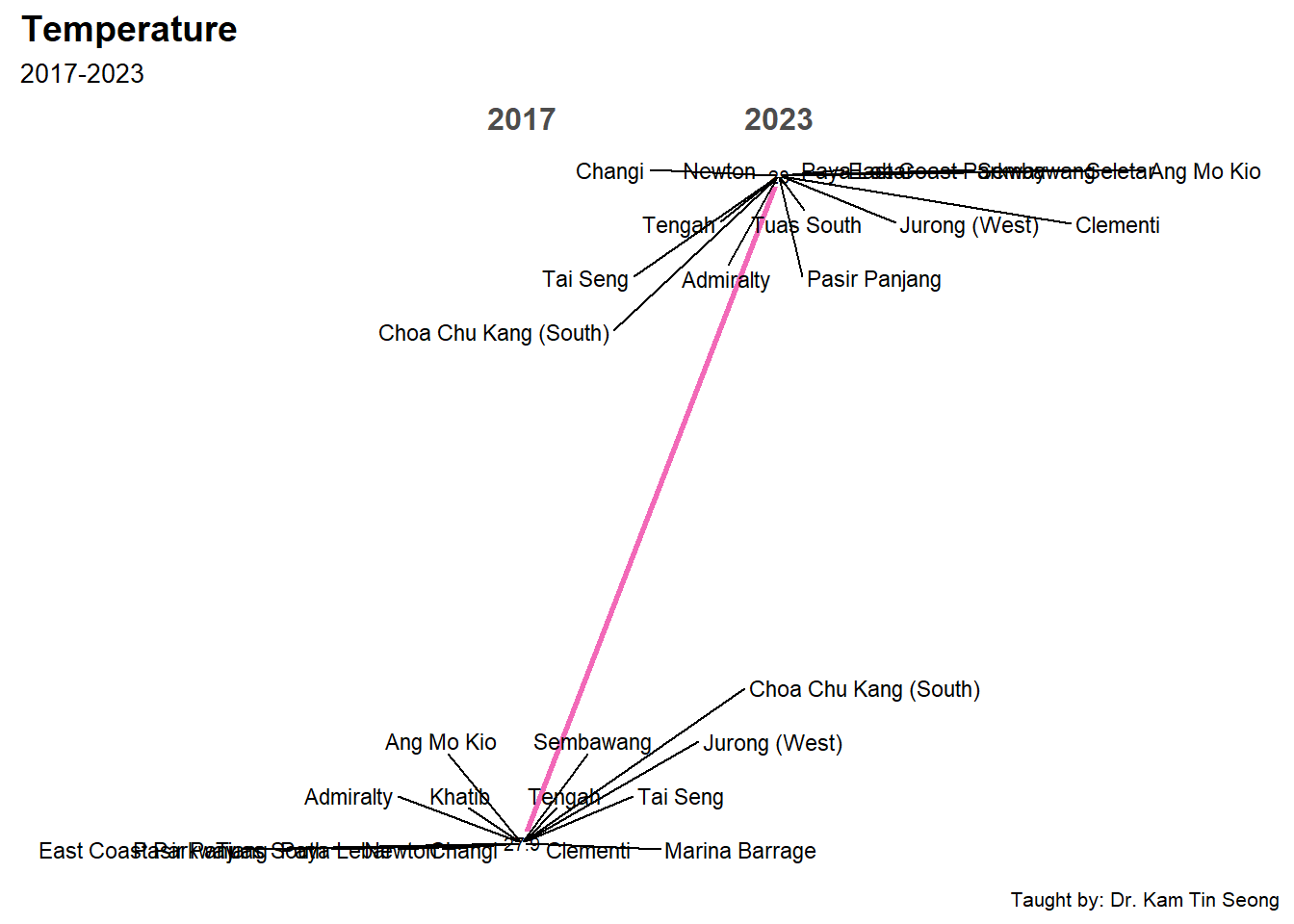

Rainfall_YM %>% 
  mutate(Year = factor(Year), 
         Station = factor(Station)) %>%
  filter(Year %in% c(2017, 2023)) %>%
  newggslopegraph(Year, MeanRainfall_Year, Station,
                  Title = "Rainfall",
                  SubTitle = "1983-2023",
                  Caption = "Taught by: Dr. Kam Tin Seong")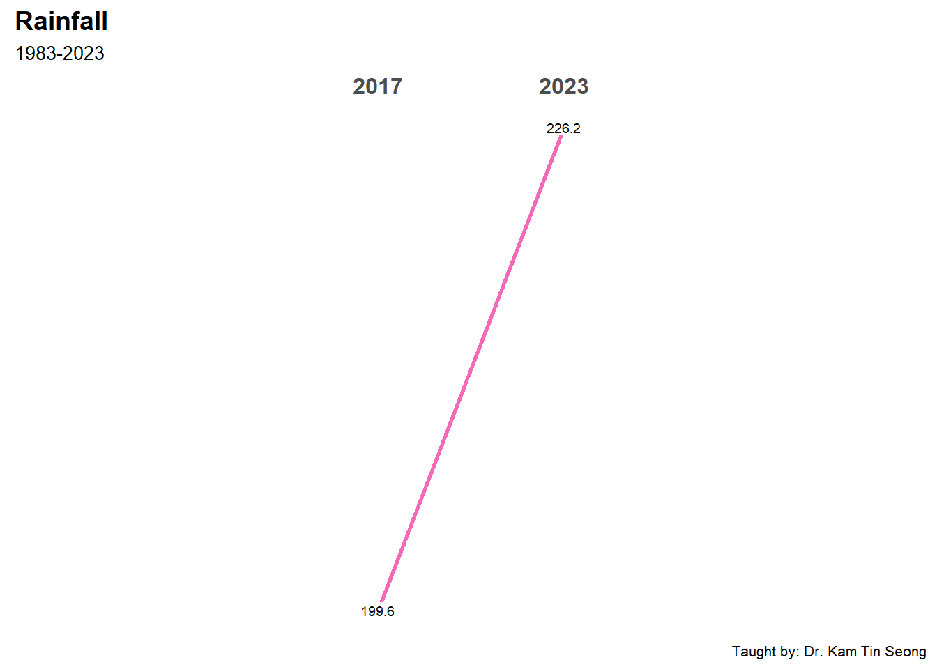

Rainfall_slope <- Rainfall_YM %>%
  select(Station, Year, MeanRainfall_Year) %>%
  distinct()

Rainfall_slope <- Rainfall_slope %>%
  mutate(Year = factor(Year))

Rainfall_slope_filtered <- Rainfall_slope %>%
  filter(Year %in% c(2017, 2023))

slope_plot <- newggslopegraph(data = Rainfall_slope_filtered,
                              Year, MeanRainfall_Year, Station,
                              Title = "Rainfall",
                              SubTitle = "2017-2023",
                              Caption = "Taught by: Dr. Kam Tin Seong")

slope_plot + geom_text_repel(aes(label = Station), size = 3, box.padding = 0.5, max.overlaps = Inf)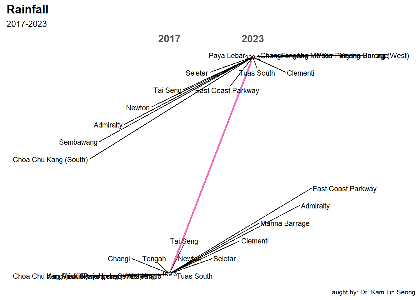

4.3 Horizon Graph

ggplot(Temp_YM) +
  geom_horizon(aes(x = Date, y = MeanTemp),
               origin = "midpoint",
               horizonscale = 6) +
  facet_grid(`Station`~.) +
  theme_few() +
  scale_fill_hcl(palette = 'RdBu') +
  theme(panel.spacing.y=unit(0, "lines"), strip.text.y = element_text(
    size = 5, angle = 0, hjust = 0),
    legend.position = 'none',
    axis.text.y = element_blank(),
    axis.text.x = element_text(size=7),
    axis.title.y = element_blank(),
    axis.title.x = element_blank(),
    axis.ticks.y = element_blank(),
    panel.border = element_blank()) +
  ggtitle('Temperature')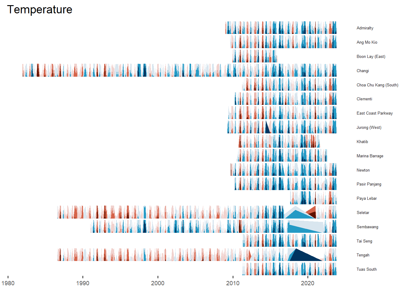

# Filter data for years 2010 to 2023
Temp_YM_filtered <- Temp_YM %>%
  filter(Year >= 2010 & Year <= 2023)

# Plot the filtered data
ggplot(Temp_YM_filtered) +
  geom_horizon(aes(x = Date, y = MeanTemp),
               origin = "midpoint",
               horizonscale = 6) +
  facet_grid(`Station`~.) +
  theme_few() +
  scale_fill_hcl(palette = 'RdBu') +
  theme(panel.spacing.y = unit(0, "lines"),
        strip.text.y = element_text(size = 5, angle = 0, hjust = 0),
        legend.position = 'none',
        axis.text.y = element_blank(),
        axis.text.x = element_text(size = 7),
        axis.title.y = element_blank(),
        axis.title.x = element_blank(),
        axis.ticks.y = element_blank(),
        panel.border = element_blank()) +
  ggtitle('Temperature, 2010-2023')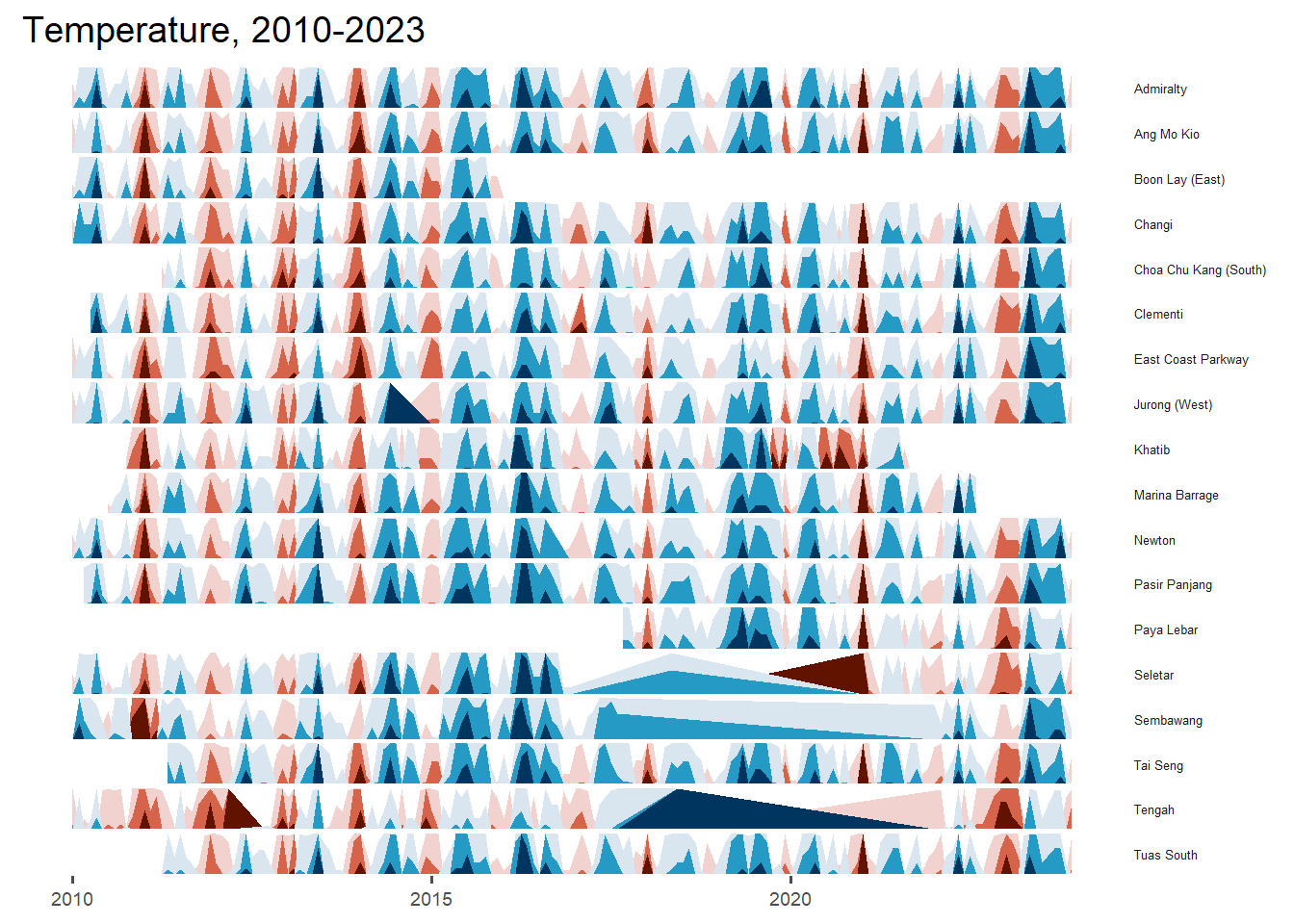

# Filter data for years 2010 to 2023
Temp_YM_filtered <- Temp_YM %>%
  filter(Year >= 2010 & Year <= 2023)

# Plot the filtered data
ggplot(Temp_YM_filtered) +
  geom_horizon(aes(x = Date, y = MeanTemp),
               origin = "midpoint",
               horizonscale = 6) +
  facet_grid(`Region`~.) +
  theme_few() +
  scale_fill_hcl(palette = 'RdBu') +
  theme(panel.spacing.y = unit(0, "lines"),
        strip.text.y = element_text(size = 5, angle = 0, hjust = 0),
        legend.position = 'none',
        axis.text.y = element_blank(),
        axis.text.x = element_text(size = 7),
        axis.title.y = element_blank(),
        axis.title.x = element_blank(),
        axis.ticks.y = element_blank(),
        panel.border = element_blank()) +
  ggtitle('Temperature, 2010-2023')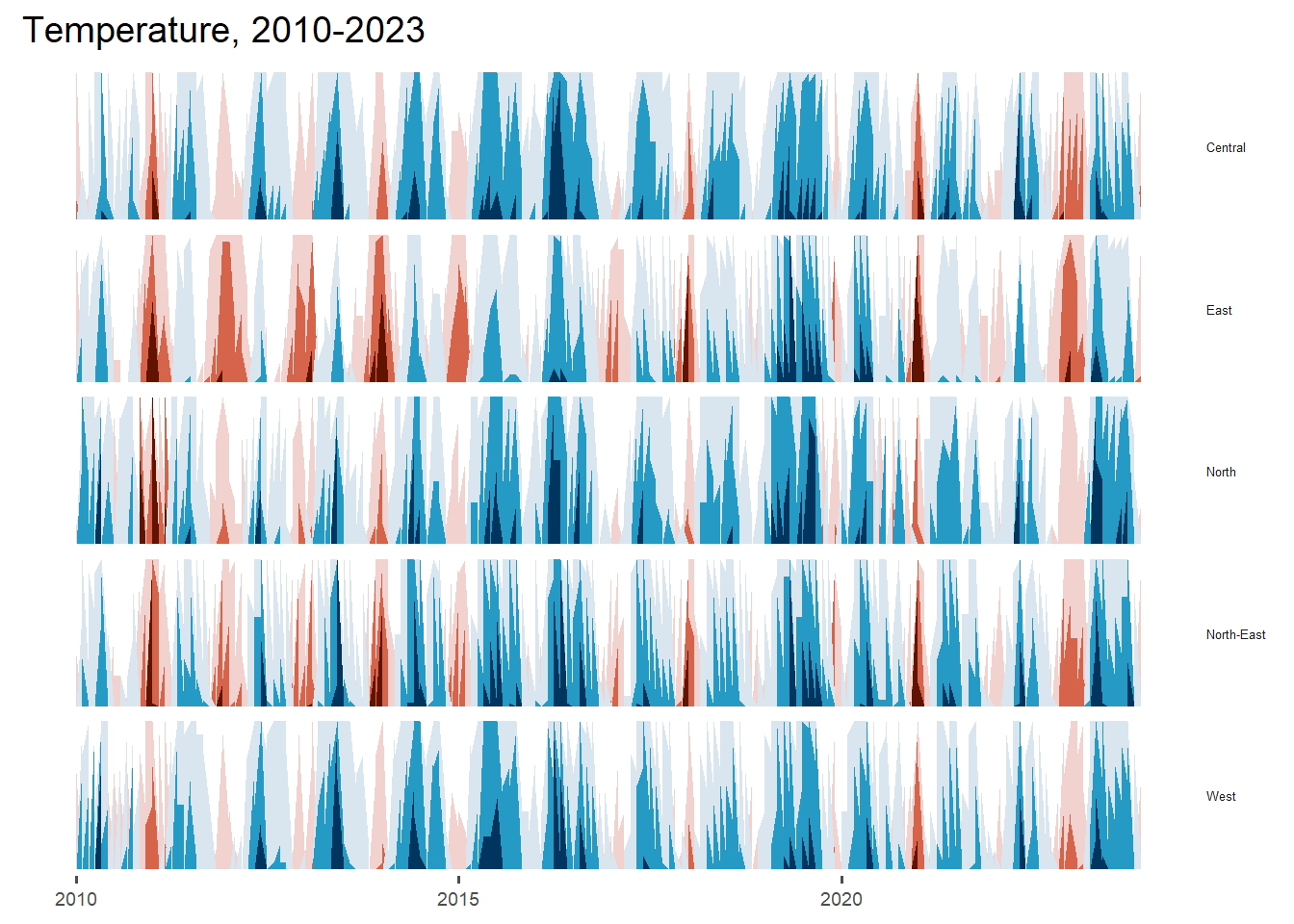

ggplot(Rainfall_YM) +
  geom_horizon(aes(x = Date, y = TotalRainfall),
               origin = "midpoint",
               horizonscale = 6) +
  facet_grid(`Station`~.) +
  theme_few() +
  scale_fill_hcl(palette = 'RdBu') +
  theme(panel.spacing.y=unit(0, "lines"), strip.text.y = element_text(
    size = 5, angle = 0, hjust = 0),
    legend.position = 'none',
    axis.text.y = element_blank(),
    axis.text.x = element_text(size=7),
    axis.title.y = element_blank(),
    axis.title.x = element_blank(),
    axis.ticks.y = element_blank(),
    panel.border = element_blank()) +
  ggtitle('Rainfall')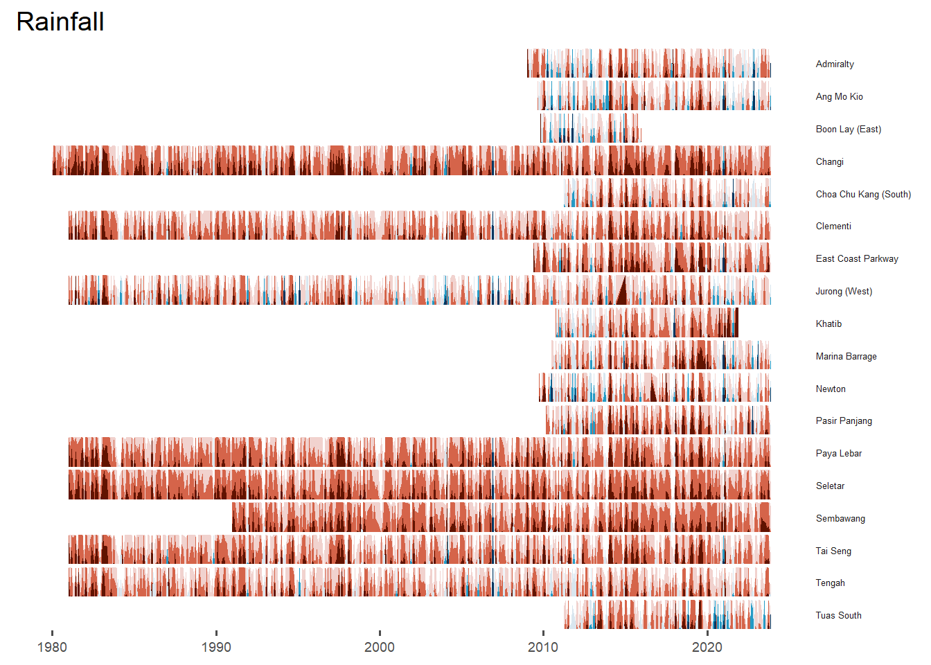

# Filter data for years 2010 to 2023
Rainfall_YM_filtered <- Rainfall_YM %>%
  filter(Year >= 2010 & Year <= 2023)

# Plot the filtered data
ggplot(Rainfall_YM_filtered) +
  geom_horizon(aes(x = Date, y = TotalRainfall),
               origin = "midpoint",
               horizonscale = 6) +
  facet_grid(`Station`~.) +
  theme_few() +
  scale_fill_hcl(palette = 'RdBu') +
  theme(panel.spacing.y = unit(0, "lines"),
        strip.text.y = element_text(size = 5, angle = 0, hjust = 0),
        legend.position = 'right',
        axis.text.y = element_blank(),
        axis.text.x = element_text(size = 7),
        axis.title.y = element_blank(),
        axis.title.x = element_blank(),
        axis.ticks.y = element_blank(),
        panel.border = element_blank()) +
  ggtitle('Rainfall, 2010-2023')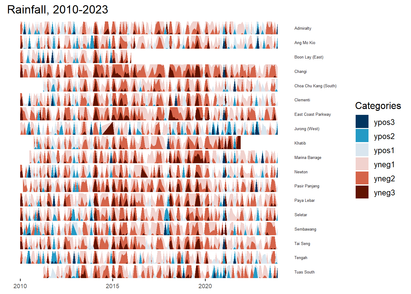

# Filter data for years 2010 to 2023
Rainfall_YM_filtered <- Rainfall_YM %>%
  filter(Year >= 2010 & Year <= 2023)

# Plot the filtered data
ggplot(Rainfall_YM_filtered) +
  geom_horizon(aes(x = Date, y = TotalRainfall),
               origin = "midpoint",
               horizonscale = 6) +
  facet_grid(`Region`~.) +
  theme_few() +
  scale_fill_hcl(palette = 'RdBu') +
  theme(panel.spacing.y = unit(0, "lines"),
        strip.text.y = element_text(size = 5, angle = 0, hjust = 0),
        legend.position = 'right',
        axis.text.y = element_blank(),
        axis.text.x = element_text(size = 7),
        axis.title.y = element_blank(),
        axis.title.x = element_blank(),
        axis.ticks.y = element_blank(),
        panel.border = element_blank()) +
  ggtitle('Rainfall, 2010-2023')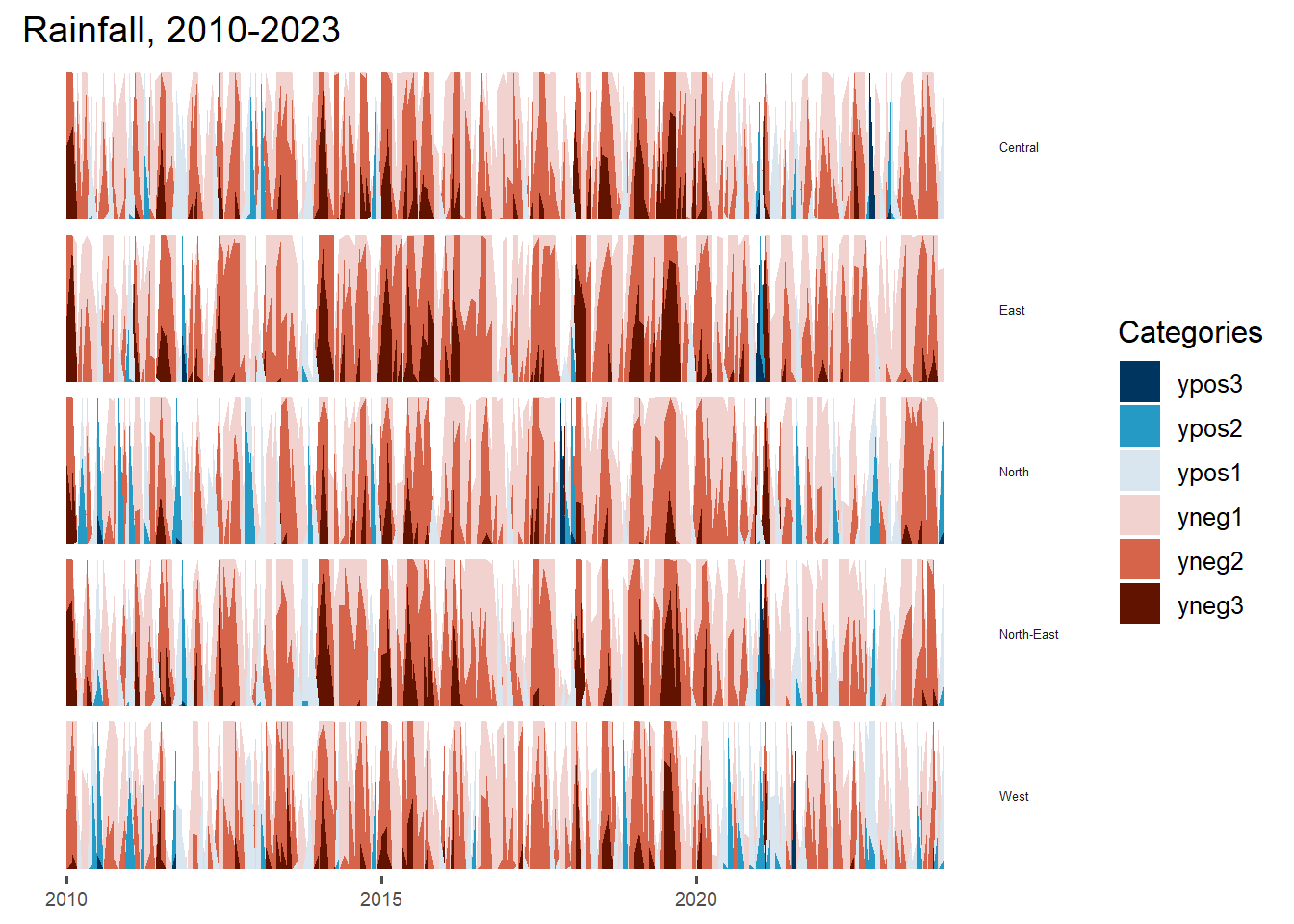

Tranformation to Shiny App

UI(fluidPage(
  
  titlePanel("Temperature and Rainfall Analysis"),
  
  sidebarLayout(
    sidebarPanel(
      selectInput("data", "Select Data:",
                  choices = c("Temperature", "Rainfall")),
      sliderInput("period", "Select Period:",
                  min = 1980, max = 2023, value = c(2010, 2023)),
      selectInput("region", "Select Region:",
                  choices = c("Region A", "Region B", "Region C")),
      selectInput("station", "Select Station:",
                  choices = c("Station 1", "Station 2", "Station 3"))
    ),
    mainPanel(
      plotOutput("plot")
    )
  )
))

Server(function(input, output) {
  
  output$plot <- renderPlot({
    # Filter data based on user inputs
    filtered_data <- filter_data(input$data, input$period[1], input$period[2],
                                 input$region, input$station)
    
    # Plotting based on filtered data
    ggplot(filtered_data) +
      geom_horizon(aes(x = Date, y = MeanTemp),
                   origin = "midpoint",
                   horizonscale = 6) +
      facet_grid(Station ~ .) +
      theme_few() +
      scale_fill_hcl(palette = 'RdBu') +
      theme(panel.spacing.y = unit(0, "lines"),
            strip.text.y = element_text(size = 5, angle = 0, hjust = 0),
            legend.position = 'none',
            axis.text.y = element_blank(),
            axis.text.x = element_text(size = 7),
            axis.title.y = element_blank(),
            axis.title.x = element_blank(),
            axis.ticks.y = element_blank(),
            panel.border = element_blank()) +
      ggtitle(paste(input$data, "(", input$period[1], "-", input$period[2], ")"))
  })
  
  # Function to filter data based on user inputs
  filter_data <- function(data_type, start_year, end_year, region, station) {
    
    Temp_YM_filtered <- Temp_YM %>%
      filter(Year >= start_year, Year <= end_year,
             Region == region, Station == station)
    
    if (data_type == "Temperature") {
      return(Temp_YM_filtered)
    }
    }
  }
)

4.4 Boxplot

Temp_YM$mean_tooltip <- c(paste0("Year: ", Temp_YM$Year,
                                   "\n Station: ", Temp_YM$Station,
                                   "\n Mean Temp: ", Temp_YM$MeanTemp, "°C"))

line <- ggplot(data = Temp_YM,
               aes(x = Year, y = MeanTemp, group = Station, color = Station, data_id = Station)) +
  geom_line_interactive(size = 1.2, alpha = 0.4) +
  geom_point_interactive(aes(tooltip = Temp_YM$mean_tooltip),
                         fill = "white", size = 1, stroke = 1, shape = 21) +
  theme_classic() +
  ylab("Annual Mean Temperature (°C)") +
  xlab("Year") +
  ggtitle("Annual Average of Mean Temperatures") +
  theme(plot.title = element_text(size = 10),
        plot.subtitle = element_text(size = 8)) 

girafe(ggobj = line, width_svg = 8, height_svg = 6 * 0.618,
       options = list(opts_hover(css = "stroke-width: 2.5; opacity: 1;"),
                      opts_hover_inv(css = "stroke-width: 1;opacity:0.6;")))

Tranformation to Shiny App

UI

ui <- fluidPage(
  titlePanel("Interactive Temperature Graph"),
  
  sidebarLayout(
    sidebarPanel(
      selectInput("station", "Select Station:", choices = unique(Temp_YM$Station)),
      sliderInput("year", "Select Year:", min = min(Temp_YM$Year), max = max(Temp_YM$Year),
                  value = c(min(Temp_YM$Year), max(Temp_YM$Year)), step = 1)
    ),
    
    mainPanel(
      plotlyOutput("temperature_plot")
    )
  )
)

Server

function(input, output) {
  filtered_data <- reactive({
    temp_year %>%
      filter(Station == input$station & Year >= input$year[1] & Year <= input$year[2])
    })
  
  output$temperature_plot <- renderPlotly({
    ggplot(data = filtered_data(), aes(x = Year, y = MeanTemp, group = Station, color = Station)) +
      geom_line(size = 1.2, alpha = 0.4) +
      geom_point(aes(text = mean_tooltip), fill = "white", size = 3, shape = 21) +
      theme_classic() +
      xlab("Year") +
      ylab("Annual Mean Temperature (°C)") +
      ggtitle("Annual Average of Mean Temperatures") +
      theme(plot.title = element_text(size = 10), plot.subtitle = element_text(size = 8))
    
    ggplotly(gg, tooltip = "text")
  })
}

4.5 Violin Plot

Temp_YM_filtered <- Temp_YM %>% 
  filter(Year == "2023")

plot_ly(data = Temp_YM_filtered,
        x = ~ Station,
        y = ~ MeanTemp,
        line = list(width=1),
        type = "violin",
        spanmode = 'hard',
        marker = list(opacity = 0.5, line = list(width = 2)),
        box = list(visible = T),
        points = 'all',
        scalemode = 'count',
        meanline = list(visible = T, color = "red"),
        color = I('#caced8'),
        marker = list(line = list(width = 2, color = '#caced8'), symbol = 'line-ns'))

Transformation to Shiny App

UI

ui <- fluidPage(
  titlePanel("Interactive Temperature Graph"),
  
  sidebarLayout(
    sidebarPanel(
      selectInput("station", "Select Station:", choices = unique(Temp_YM$Station)),
      sliderInput("year", "Select Year:", min = min(Temp_YM$Year), max = max(Temp_YM$Year),
                  value = c(min(Temp_YM$Year), max(Temp_YM$Year)), step = 1)
    ),
    
    mainPanel(
      plotlyOutput("temperature_plot")
    )
  )
)

Server

server <- function(input, output) {
  
  filtered_data <- reactive({
    Temp_YM %>%
      filter(Station == input$station & Year >= input$year[1] & Year <= input$year[2])
  })
  
  output$temperature_plot <- renderPlotly({
    gg <- ggplot(data = Temp_YM_filtered(), aes(x = Year, y = MeanTemp, group = Station, color = Station)) +
      geom_line(size = 1.2, alpha = 0.4) +
      geom_point(aes(text = mean_tooltip), fill = "white", size = 3, shape = 21) +
      theme_classic() +
      ylab("Annual Mean Temperature (°C)") +
      xlab("Year") +
      ggtitle("Annual Average of Mean Temperatures") +
      theme(plot.title = element_text(size = 10),
            plot.subtitle = element_text(size = 8))
    
    ggplotly(gg, tooltip = "text")
  })
}

4.6 Calendar Heatmap

p <- ggplot(Temp_YM, aes(x = Month, y = Year, fill = MeanTemp)) + 
  geom_tile(color = "white") + 
  theme_tufte(base_family = "Helvetica") + 
  scale_fill_gradient(low = "gold", high = "goldenrod3") +
  labs(title = "Calendar Heatmap of Mean Temperature: 2013-2023", x = "Month", y = "Year", fill = "Temperature") +
  theme_minimal() +
  theme(axis.ticks = element_blank(), 
       plot.title = element_text(hjust = 0.5),
       legend.title = element_text(size = 8),
       legend.text = element_text(size = 6) )

ggplotly(p)

References: https://cran.r-project.org/web/packages/datagovsgR/datagovsgR.pdf